In the beginning of our learning about electronics we concentrate on RLC components - Resistors, Capacitors and Inductors before moving on to study transistors and diodes. Possibly studying transformers a bit along the way. It would have been better to spend longer on the passive components.
To learn that resistors are not just things obeying Ohm's law; R = V/I (Ohms are simply volts per amp). This is only true as a first approximation - once current begins to flow the resistor heats up - and invariably its resistance changes for each degree of temperature rise. The wires of a resistance possess inductance, maybe 20 to 50 nH per inch. And there is a capacitance or two present as well!
Capacitors are not that simple either; A lot of types of modern small capacitors have capacitance values that vary dramatically as the DC voltage across them varies. Larger, older capacitors have only a nominal value - +80/-20% - a so called 10,000uF electrolytic capacitor can be anywhere between 8000 and 18,000 uF in value. And it ages, so after a year or so its value has changed, more so if operated in an elevated temperature. And after 20-30 years you need to throw them out and replace them - they have dried out (this is how you fix old valve gear). Their value also depends on the frequency of any AC passing through it, and just to make life complicated this is a voltage dependent effect. Luckily a lot of modern circuits don't care what value the capacitance is as long as it has a low effective series resistance (ESR).
Of course it does depend on how the capacitor was made - its type. I sometimes think a degree in chemistry would be useful in remembering all the different materials and constructions that modern (and old) capacitors used.
So much to learn and so little time.
And then we come to inductors. These can be;
- Air-Cored spiral -wound like a cylinder
- Wound on a magnetic core in the shape of an; E, or U either solid or built up from flat laminations
- Wound on a round pot core
- Wound on a rod, there are several ways to wind the turns too, and different types of wire
- a flat pack with a slit or mounted over a set of turns laid down on a flat substrate (e.g SMD inductors or inductors made of PCB material
- a cylinder with one, two or six holes or
- a ring/doughnut structure (which to be fair is the same as a cylinder with one hole.)
The material can vary from various irons through to ceramics of nickel, zinc, manganese.
The applications can use;
- DC,
- low frequency AC such as 50 or 60 Hz
- Slightly higher frequencies up to 100kHz and lately to nearly a Megahertz for switching power supplies and battery chargers.
- Also radio frequencies that are lowish, under 3MHz or
- In the radio bands we use for High Frequency communications (3 to 30MHz) or
- very and even ultra high - VHF/UHF as well as
- microwaves as found in mobile phones, satellite dishes and microwave (sic) ovens.
- I suppose the millimetre waves of 5G must use inductance, not sure we'd recognise them.
We need to "manage the complexity" and as humans we abstract the truth to things that are easier to work with. Thus we use Ohms law and formula for the impedance (Reactance) of coils and capacitors and can work out approximate voltages and currents for networks of components. We use "ideal" components, we assume everything is linear - is well behaved with no second order effects.
Complicated networks can sometimes be simplified by applying the formula for series and parallel components, sometimes with star to delta conversions or by judicious use of Kirchoff's Voltage and Current laws or conversions using Thevenin or Norton equivalent circuits. You might end up having to solve simultaneous equations, or you can create enormous matrices and then have to do Matrix inversions and other Matrix arithmetic
All good stuff, and why it takes 3 or 4 years to make an electronics engineer.
Instead you can let the computer do the heavy lifting. Modelling and Simulation programs are now vital tools for a practising engineer. You can not expect to manually solve the problems in a finite time span and are obliged to use a computer. Spreadsheets are also useful, particularly with their complex number formula. Spreadsheets make smart people smarter, although...
The most famous/often used circuit modelling packages are based on the free and open source SPICE program that came originally from Berkeley University in 1973. The name SPICE stands for Simulation Program (with) Integrated Circuit Emphasis but it can be applied in a number of applications. There are several important SPICEs available. The Linear Technology Company (now owned by Analog Devices -ADI) give away LTspice at no charge. The free, open source KICAD Schematic Capture (circuit drawing) and PCB layout tools package includes NGSpice and the MicroCap software is now given away free (used to cost thousands of pounds but the owner has retired and has been most benevolent in allowing anyone to use MicroCAP free). The URLs are below. There are also spice programs available to purchase - PSpice does have a 30 day trial version available (and a restricted free version) and is quite popular in Universities, they also use HSpice and other very expensive packages. There are a number of textbooks on LTspice and Pspice available on Amazon and support forums and Youtube videos for both available online. There is little to choose between them, I find LTspice easier and quicker to learn and it has many more downloads than any of the others, so presumably it is much more popular.
Downloads:
As a trained engineer I was taught to calculate voltages and currents around simple transistor circuits. To do this we pretend the transistor is a sub circuit of resistors and capacitors and voltage and current sources that are dependent on some external value. I realised it was all over one day when I looked into how SPICE calculates transistor models. I was using 3 components per transistor at lowish frequencies, rising to maybe 8 or 9 at radio frequencies. I discovered that there were 54 different parts to the transistor models that SPICE was using when it calculated circuit values. We can't compete, the machine has won.
You can use the package to;
- Work out the DC operating point (no signal applied) - the values at various nodes around a circuit to help you fault-find and check the bias conditions have been calculated correctly.
- Work out "small signal" performances; gain and frequency responses are obvious examples, but also the input and output impedances (and how these vary with frequency) - this is important when you interface two modules together.
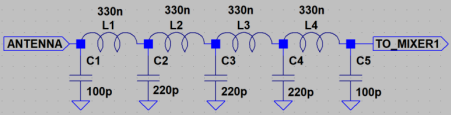
- Design filters and see how changing a components value to a standard value affects performance. (there are even tools that can generate LTSpice files by filling in a form about what type of filter you want - see http://www.tonnesoftware.com/elsie.html or other tonnesoftware programs)
- Work out how much noise a circuit produces. I want to experiment with this...I am a bit dubious about how accurate the noise data included in some transistor models by manufacturers are, whilst microwave transistor models may be accurate I think a lot of ordinary transistors have nominal or even missing noise parameters in their models.
- Work out what the maximum output can be before clipping, Usually either the "one dB compression point" or the third order intercept point (IIP3 or OIP3) or even THD.
- Calculate what harmonics are produced.
- Work out the power consumed or how much power each component dissipates.
- Calculate the temperature rises in a circuit and its effects.
- Of less use to amateurs perhaps - but you can vary every component randomly about its tolerance values - this tells you that if you build a thousand circuit boards, how many will pass or fail some output test. - known as Monte Carlo testing. You can use this to see if building a filter using 5% tolerance components is likely to give a reasonable performance.
The ubitx (and earlier singleband Bitx) was designed by Ashhar Farhan VU2ESE from India. A superb designer. He has also published a Youtube video which I found inspirational; it covers the design, building and testing of a simple feedback amplifier - a single transistor circuit that is the basis for all his RF low signal amplifiers. Understand it and you can understand nearly all the others.
The video discusses the circuit, then he solders the components on a small piece of copper PCB material - blank, un-etched copper (single or double-sided). He solders one leg of a component down to the board if it is to be wired to "earth" or 0 volts. This leaves enough legs sticking up in the air to solder other component between them - the entire circuit is wired up in about 2 minutes! This is known as ugly construction and whilst not pretty, is actually very effective at radio frequencies. He adds a couple of BNC connectors and a power jack and powers up the circuit. His only test gear is a $100 homebrew antuino - he designed this antenna analyser but it can also "receive" signals and plot their amplitude. A £35 NanoVNA would do instead.
He shows you how to measure the gain, the input impedance and output impedance and how they vary with frequency as well as the maximum amount of signal the amplifier can accept before generating distortion. These parameters define nearly everything about the amplifier (with the exception of noise figure and some phase data)
Gain 17dB drooping slightly at VHF
Input SWR and output SWR - the antuino can measure return losses or SWR.
50 Ohm input impedance, Rin - a NanoVNA can gives Zin directly.
50 Ohm output impedance. Rout - though by measuring Return loss we can estimate Zout
Input third order Intermodulation distortion (IMD) Products of +8dBm, this is called the IIP3
Anyone interested in homebrewing radio circuits must watch this 51 minute video
I have put the circuit into LTspice and simulated it - and got the same results as the physical measurements (always a relief!) and may create a powerpoint presentation or Youtube video - as much as an example of how to use LTspice as well as being a useful adjunct to Farhhan's work.
There are a number of simulation runs in the video/powerpoint;
- Applying a sine wave signal and seeing the output - much as a signal generator and scope would.
- measuring voltage gain using this - noting Vin and Vout. Calculating Power gain in dB.
- varying the input until we can see (qualitatively) when distortion and clipping is occuring.
- Measuring input voltage and current to get input impedance (with output terminated in 50 Ohm)
- Measuring output impedance by applying a signal to the output and measuring its V & I.
- A better way to measure gain, Zin and Zout using "two port analysis" - the .NET command
- Measuring the Noise Figure - as I said above, I am dubious as to the accuracy and presence of noise data in the models of many transistors but the results are plausible. Hard to measure physically to verify. If I can't get a calibrated noise source soon I may need a thermos flask of liquid Nitrogen - but that's another story.
- Distortion; I had bother here, I did the same two tone test that Farhhan does but my results were initially suspect. I had to use the FFT function in LTspice and lean heavily on the way data is gathered in the package. I got it working with considerable help from the LTspice forum at groups.io (
https://groups.io/g/LTspice ) (the secret was to have a tiny "timestamp" which meant it took 40 minutes and several gig of diskspace to run the simulation!
Most of the time we use the .TRAN and
the .AC analyses of SPICE.
A .TRAN analysis runs for a fixed time
period from startup and uses numerical techniques to calculate
voltages and currents at every node using large signal/non-linear
models of the components. The .AC analysis works out the .DC
operating condition and then creates a small signal/linear model of
the circuit at that bias point. It applies a single frequency sine
wave, calculates the V and I assuming linear operation, changes the
frequency of the input signal and repeats the process. It sweeps the
input across a frequency range and is useful to see frequency
response. It is using an approximation of the actual circuit but is
useful nonetheless.
Quote from groups.io LTspice forum
"Small
Signal Analysis takes a system, and linearizes it about its operating
point, and because the system it looks at is a linear system, there
are a lot of powerful techniques that can be used to very precisely
analysis the system, and often get closed form mathematical results.
(But the precise answers are to an approximation of the system).
Large
Signal Analysis, uses a much more detailed model of the system,
including non-linearities. Because of this, you rarely get
significant closed form mathematical results, but the systems tend to
(be)
processed
with numeric methods. These answers tend to be approximations, but to
a much better model of the system, so can be more accurate."
And a further quote
"an
.AC analysis in SPICE, ... SPICE converts those transistor and diode
models into their small-signal (linear) equivalents at the DC
operating point of your circuit, and all results from that point
forward are based on that. Even if your simulation uses 10KV AC
signals, the diode and transistor models in that .AC simulation are
small-signal models because they've been linearized. But they
were linearized starting with the original nonlinear (large-signal)
models.
In
a .TRAN analysis, the simulation uses the full nonlinear model so it
works for small and large signals."
And
"One common
way to determine whether a signal is small enough to be “small
signal” is to do a transient (.TRAN) analysis using a sine signal
source. Then, you can do a Fourier Analysis of the output. One of the
metrics of this analysis is a harmonic distortion number. You can
then vary the amplitude of your input signal until the harmonic
distortion is “small enough”. At this point, for your
application, it is then Small Signal."
LTspice can calculate THD (total
harmonic distortion) which suits audio amplifier designers. RF
designers work with third order distortion rather than the total
distortion as it is usually the biggest and our circuits have
filters or we are only interested in outputs around a single
frequency or frequency band. The distortion due to third order
products should increase rapidly as the input rises (three times more
rapidly). You can test for this by applying two similar tones f1 and
f2 at a certain level and use the FFT function to see the distortion
(2f1-f2 or 2f2-f1). i.e if you apply 0 dBm tones and get 2f1-f2 at
-46 dB below that and then increase the inputs to 3 dBm you should
see f2-f1 at 9dB higher or -40dB below the tones. My initial run of
LTspice did not do this. I was not setting the FFT parameters
correctly and others have noted "funnies" in the FFT
results. Gunthard Kraus simulates an entire 137MHz satellite
receiver (convertor) using LTspice
at http://www.gunthard-kraus.de/LTSwitcherCAD/SwitcherCAD-Tutorial_English/pdf-File/ When
I noticed this I went on to assess IMD a different way - If you apply
a signal and then increase its strength, there comes a point when the
amplifier cannot amplify enough and the gain starts to drop, a
standard value is when the gain drops one dB from its theoretical
value. the "one dB compression point" POUT(-1dB). The OIP3
figure tends to be 13 to 15dB above this value in BJT amplifers and
about 10-12 dB in FET circuits. This gave me an alternative way of
estimating OIP3.
In parallel with this work I asked for
help on the forum, Tony Casy, Andy, Vlad and Dana all replied (it is
a really good group) and gave me FFT settings that finally gave
believable results - I could see third order products rise three
times faster than rises in the input - which is correct behaviour and
also the OIP3 were about 15dB higher than the 1dB compression point
which further reassures me the results can be trusted. Tony also
created a version of one of my models to present automated results of
compression, it uses a lot of LTspice commands but a lovely example
of what a "power user" can do
See my Youtube videos when they go up
as there is a lot of fiddly bits to get it all working - spread over
8 different LTspice simulation runs. They are a good example of how
to use simulation as a design tool when designing, or before
building, homebrew transistor circuits to be used a amplifiers as
part of receivers and transmitters.
Of course LTspice is also very very
useful for filters and other radio circuits. When I get around to
simulating the uBitx I will be simulating mixers, filters and audio
circuits - hopefully everything!. I have a simulating model of a ring
mixer already and it works - the computer gives the same answer as
the theory and the same results as a real circuit. One wrinkle to the
model is that all 4 diodes have the same model parameters -
absolutely identical. In real life, if you pick up 4 diodes they all
differ slightly, we often manually match them by picking 4 from a
larger batch so that they have the same forward voltage drop maybe
within a millivolt or two (at a chosen fixed forward current -
perhaps what the diode test function on your DVM uses!). This is
important - as a first approximation, but of course the question is -
are they still matched at differing currents and what happens when
the ambient temperature increases? This is an example of when you
need to do multiple runs at slightly different conditions. In LTspice
this can be done by using Monte Carlo simulations and these can take
a lot of time - I shall be running my computers overnight or longer
to get results for this one. It will have to wait until I am actually
building my uBitx however and I will create detailed diode models
from the few hundred diodes in my junk box by measurement.
No manufacturer publishes the data that
I need to see the statistical tolerance spreads on the parameters -
they usually just publish a single figure, or at best (but very
rarely) the three figures of minimum, typical and maximum. I need the
standard deviations of each published parameter (assuming a normal
bell curve spread of values). This is way beyond what a hobbyist
radio amateur needs but I find it interesting and the current
situation is giving me time to be thorough. (Not sure if it is the
lockdown or the fact I am recently retired)